Chapter 12 Introduction to Excel
Vocabulary
Adjacent: Close to or next to.
Cell: A single box on a table or spreadsheet that can contain text (e.g., letters, numbers, dates).
Cell reference: A unique name or address of cell that is based on a set of coordinates that a cell occupies on a worksheet. For example, a cell that appears in column C and in Row 8 is C8.
Column: The vertical series of cells separated by lines or space from other vertical series of cells and found in a table or spreadsheet.
Column heading: Also known as column headers. The shaded area at the top of the column and contains a letter or a series of letters (e.g., XA, BB). By clicking the column header, the user selects the entire column. The column width can be changed by dragging the line to the right of the heading.
Fill handle: A tool indicated by a plus sign cursor that is observed when the user moves the cursor to the bottom right corner of a selected cell or cell range in Excel. This tool is used to fill or extend a series or data.
Formula: A mathematical equation in a spreadsheet that performs a calculation and shows the result in a cell.
Function: A predefined formula in a spreadsheet that performs a calculation with specific values.
Hover over: Moving the mouse pointer over an option without selecting it.
Row: The horizontal series of cells separated by lines or space form other horizontal series of cells and found in a table or spreadsheet.
Row heading: Also called row header. The shaded area at the left side of each row. By clicking the row header, the user selects the entire row. The row height can be changed by dragging the line below the row heading.
Select: To highlight a cell or multiple cells (cell range) and the next command will impact these cells.
Workbook: A spreadsheet program file created in MS Excel and has the file extension .xls or .xlsx. Contains one or more worksheets.
Worksheet: Found within a workbook; also called a spreadsheet. Consists of cells that can contain data, formulas, and functions.
Introduction
Excel is a spreadsheet program and can be used for the following:
- Store and organize information such as supply and inventory lists.
- Analyze information, such as budgets, revenue, and expenditure.
Each Excel file is considered a workbook. Each workbook has one or more worksheets. When the user opens Excel, the Excel Start Screen appears (Figure 1). The user can open an existing workbook, select a template, or select a new workbook. To select a blank worksheet, use the keyboard shortcut keys (Ctrl + N).
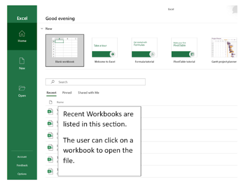
The Excel Window
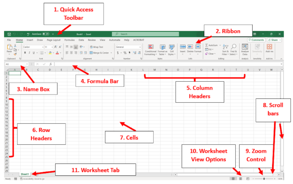
Several of the features of the Excel window are the same as Microsoft Word (Figure 2A). This includes the Quick Access toolbar and the Zoom Control. The format of the ribbon and tabs are also like Word, though different controls are available. The following describes some of the features of the Excel window:
- Quick Access Toolbar: Provides frequent commands in one convenient location for the user regardless of the tab being used.
- Ribbon: Provides commands and options for the user to select.
- Name Box: Indicates the location or name of the selected cell. The name of a cell includes a letter followed by a number. The letter represents column of the selected cell, and the number relates to the row.
- Formula Bar: Allows the user to enter and edit data, or to add a function or formula to the cell.
- Column Headers: Found above Row 1. A column header is at the top of each column. Each column is identified by a letter (A, B, C). A column is composed of a group of cells that run vertically (top to bottom) on the spreadsheet. The column headers can be hidden by selecting the View tab and clicking to remove the checkmark in front of Headings in the Show group (Figure 2B). Both the row and column headers will be removed. To add the headers, click to add a checkmark in front of Headings in the Show group.
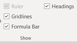
Figure 2B. The Show group on the View tab. - Row Headers: Found to the left of Column A. A row header is at the start of each row. A row is identified by a number (1, 2, 3). A row is composed of a group of cells that run horizontally (left to right) on the spreadsheet. The row headers can be hidden by selecting the View tab and clicking to remove the checkmark to the left of headings in the Show group (Figure 2B).
- Cells: Are rectangular boxes in the spreadsheet. Each cell has a unique name or address, called a cell reference, which is based on its location (the column and row). The cell reference is a combination of its column and row (e.g., A1, B3). The user can click a cell to select it.
- Scroll Bars: Consist of vertical and horizontal bars that can be used to move through the worksheet.
- Zoom Control: Allows the user to move the slider to use the zoom control tool. The zoom percentage is located in the lower right corner of the window.
- Worksheet View Options: Provides three views for the user to select from when viewing the spreadsheet. These views are also available on the View tab in the Workbook Views group. The three views available in the lower corner of the Excel window are as follows:
- Normal view: This is the default view for Excel worksheets.
- Page Layout view: This shows how the worksheet will appear when it is printed. The user can add footers and headers in this view.
- Page Break Preview: The user can modify the location of the page breaks using this view.
- Worksheet Tabs: Are used to view the worksheets within the workbook. The user can click a tab to view another worksheet.
Working Within a Worksheet
To work within a worksheet, the user needs to know how to navigate in the worksheet, select cells, copy and paste content, and insert and delete cells. Learning how to modify columns, rows, and cells is also helpful when using a worksheet. This section describes these skills.
Navigating in a Worksheet
To move through the worksheet, the arrow keys and several keyboard shortcuts can be used. The four arrow keys can also be used to move from cell to cell in a worksheet. The Up arrow key moves one cell up, and the Down arrow key moves one cell down. The left arrow key moves one cell to the left, and the right arrow key moves one cell to the right.
Use these keyboard shortcut keys to navigate a worksheet:
- To move to the cell to the right, press the Tab key.
- To move to the cell to the left, use the Shift + Tab keys.
- To move to the next row, press the Enter key.
- To move to the prior row, use the Shift + Enter keys.
- To move to the last cell used on the worksheet (the cell in the lowest row and to the farthest right column), use the keyboard shortcut keys (Ctrl + End).
- To move to the first cell of the worksheet, use the keyboard shortcut keys (Ctrl + Home).
Selecting Cells in a Worksheet
A cell needs to be selected to enter data, a formula, or a function. To select a cell, click on the cell using the cursor/pointer or use the arrow keys or keyboard shortcut keys. When a cell is selected, borders will appear around the cell (Figure 3A). The selected cell’s reference will appear in the name box (Figure 2A). The row heading and the column heading will also be highlighted. The cell will be selected until another cell is selected.
If multiple adjacent cells need to be selected: Select a cell and then hold down the left click button on the mouse while dragging over the other cells that need to be selected.
If multiple non-adjacent cells need to be selected: Hold the Ctrl key while selecting the cells.
To select an entire column: Click the letter at the top of the column. The same result can be achieved by selecting a cell in the column and then pressing the keyboard shortcut keys (Ctrl + Space). To select non-adjacent columns, press the Ctrl key while selecting the column numbers.
To select an entire row: Click the number in front of the row. The same result can be achieved by selecting a cell in the row and then pressing the keyboard shortcut keys (Shift + Space). To select non-adjacent rows, press the Ctrl key while selecting the row numbers.
To select the entire worksheet: Click the Select All button above the 1 and to the left of the A column (Figures 3B and 3C). To unselect the entire worksheet, click into any cell of the worksheet.
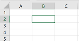


Cell Range
Often the user must select multiple cells. A cell range is a group of cells. A cell range is identified by the first and last cell of the range. These two cells are separated by a colon. For example, if the user selected the first three cells in Columns A and B, the cell range would be A1:B3. This cell range includes the following cells: A1, A2, A3, B1, B2, and B3.
Add, Edit, and Delete Content
A user can add content to the cells of a worksheet. The content can include text (i.e., letters, numbers, and dates). Formulas, functions, and formatting can also be added to cells. (Formulas and functions will be discussed in the next chapter.)
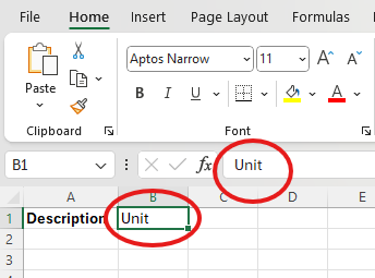
To add content to a cell: Select the cell (by clicking on it). Type the content either in the cell or in the formula bar. Press the Enter key to move to another cell. The content will appear in both the cell and the formula bar (Figure 4A).
To overwrite the content in a cell: Click the cell and type the new content. The prior content will be deleted.
To edit content in a cell: One of two methods can be used. Double-click the cell and the cursor will flash in the cell. The user can edit the content in the cell. The other method involves clicking on the cell to select it. The contents of the cell will be visible in the formula bar. The user can click in the formula bar, make revisions to the cell content, and then click the Enter key.
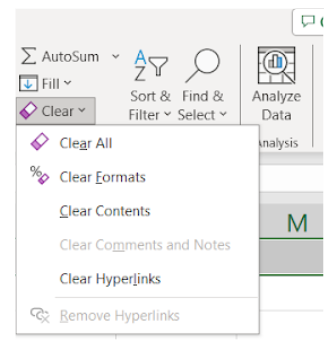
To delete the content of a cell or multiple cells: Select the cell(s). Press the Delete key or use the Clear command to delete content from one or more cells. To use the Clear command, select the Clear button in the Editing group on the Home tab. Select Clear Content (Figure 4B). (The Clear command can also be used to clear hyperlinks, formatting, or everything in the cell.) The Backspace key can be used to delete content from a cell, but it will only delete content for one cell even if multiple cells are selected.
Cut, Copy, and Paste Tools
Content from cells can be cut or copied and pasted into other cells. When cutting content from a cell and pasting it into another cell, the content is moved. Copying content from one cell and pasting it into another cell duplicates the content.
To cut content from a cell(s): Select the cell(s). Click the Cut command in the Clipboard group on the Home Tab, use the keyboard shortcut keys (Ctrl + X), or right click and select Cut. This content can then be pasted into another cell(s).
To copy the content: Select the cell(s) to copy. Click the Copy command in the Clipboard group on the Home Tab, use the keyboard shortcut keys (Ctrl + C), or right click and select Copy. The copied cell(s) will have a dashed border around it. This content can then be pasted into another cell(s).
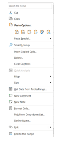
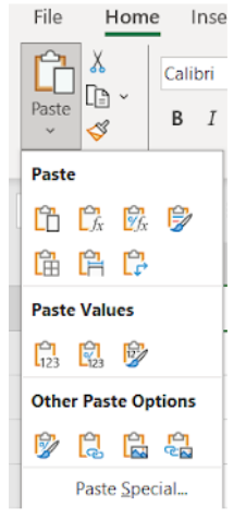
To paste the content: Select the cell(s) where the content is to be pasted. Click the Paste command in the Clipboard group on the Home Tab, use the keyboard shortcut keys (Ctrl + V), or right click and select a Paste Option (Figure 5A). Additional paste options are available on the Paste menu and can vary depending on the cell copied. Options can include formulas, formatting, and borders (Figure 5B).
Drag and Drop Cells
Content of cells can be moved to other cells by using the drag and drop method. This relocates the content and does not duplicate it.
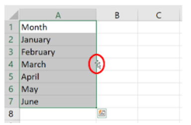
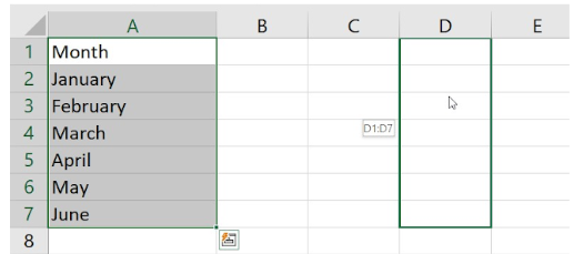
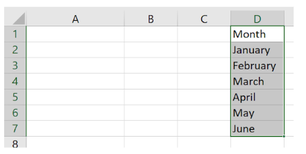
To use, select the cell(s) to be moved. Hover the pointer over the border of the selected cell(s). When the pointer changes to a pointer with four arrows, click and drag the cell(s) to a new location (Figure 6A). During the dragging process, a box appears with thick borders (Figure 6B). Once the box is in the desired position, release the mouse click button. The content selected will drop (fill) into the new cells (Figure 6C). In the Figures 6A-6C, A1:A7 were dragged to D1:D7.
Fill Handles
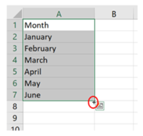
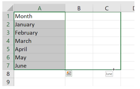
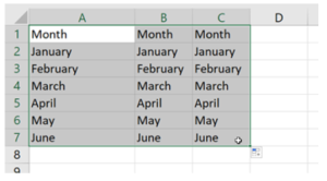
If content needs to be copied to additional adjoining cells, the fill handles can be used. To use this method, select the cells to be copied. Hover over the lower right corner of the last cell copied. When the fill handle appears, click and drag the handle until all of the cells to be filled with the content are selected (Figures 7A and 7B). Release the mouse click button, and the cells are filled with the content (Figure 7C).
In Figure 7A, A1:A7 were selected. The fill handle was dragged to include B1:C7 (Figure 7B). The content from A1:A7 filled into B1:C7 (Figure 7C).
Extend Series Using the Fill Handle
When working with a series, Excel can continue the series if the fill handle is used. For instance, if a row or column contains a numeric sequential order, the days of the week, or months of the year, the fill handle can complete the series. Usually, several cells of a sequential order are needed for Excel to complete the series.
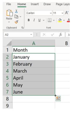
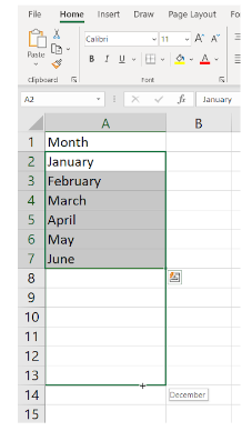
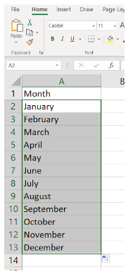
To use this feature, select a cell range you wish to continue (Figure 8A). Click and drag the fill handles to extend the series (Figure 8B). Release the mouse click button, and the selected cells will be completed with the series (Figure 8C).
In the following figures, the first six months of the year were selected (Figure 8A). Six additional cells were selected, and Excel indicated the month to fill in the last cell (December) (Figure 8B). Figure 8C shows the additional months filled in by Excel.
Modify Cells, Rows, and Columns
By default, cells have the same height and width throughout the worksheet. The user can modify the column width and row height. Cells, rows, and columns can be deleted and inserted. Columns and rows can be hidden or unhid. Cells can be merged and unmerged. This section discusses these worksheet modifications.
Change the Column Width
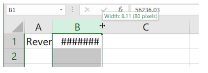
When a column is not wide enough to show the entire number in the cell, the content is displayed with pound signs (#######) (Figure 9A). Once the column is enlarged, the complete number will be seen.
Use these techniques to change the column width:
- Adjust the column line in the column heading: Position the pointer over the column line in the header. When the pointer becomes a double arrow, click and drag the mouse to the left to decrease the width or to the right to increase the width of the column (Figure 9A). When the mouse click button is released, the width will change.
- Use the AutoFit tool: The AutoFit tool will automatically modify the column width, so it fits the content. To use the AutoFit tool, position the pointer over the column line in the header. When the pointer becomes a double arrow, double (left) click the mouse. This will automatically change the column width, so it fits the content. To AutoFit several columns at once, select the columns to modify and do one of the two methods:
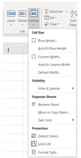
- On the Home tab, click the Format command in the Cell group. The Format dropdown menu appears (Figure 9B). Select AutoFit Column Width, and the selected columns will be resized.
- Double-click on any of the column lines that were selected, and all of the selected columns will be resized.
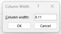
- Use the Column Width tool: To set the column width to a certain number, select the column(s) to be modified. On the Home tab, click the Format command in the Cell group. Select Column Width on the dropdown menu. When the Column Width dialog box appears, type in the width measurement and click OK (Figure 9C). The column width size appears when a person hovers over and clicks the column line in the column heading (Figure 9D).
- Apply a uniform column width size to the entire worksheet: To make all of the columns the same width, click the Select All button (found below the name box). Position the pointer over the column line in the header. When the pointer becomes a double arrow, click and drag the mouse to either decrease or increase the width of the column. When the mouse click button is released, the width will change on all of the columns.

Change the Row Height
These are the ways to change the row height:
- Adjust the row line in the row heading: Position the pointer over the row line in the header. When the pointer becomes a double arrow, click and drag the mouse to either decrease or increase the height of the row. When the mouse click button is released, the height will change.
- Use the AutoFit tool: To AutoFit a row or several rows at once, select the row(s) to modify. On the Home tab, click the Format command in the Cell group. The Format dropdown menu appears. Select AutoFit Row Height (Figure 9B).
- Use the Row Height tool: To set the row height to a certain number, select the row(s) to be modified. On the Home tab, click the Format command in the Cell group. When the Format dropdown menu appears, select Row Height (Figure 9B). When the Row Height dialog box appears, type in the height measurement and click OK. The row height size appears when a person hovers over and clicks the row line in the row heading.
- Apply a uniform row height size to the entire worksheet: To make all of the rows the same height, click the Select All button (found below the name box). Position the pointer over the row line in the header. When the pointer becomes a double arrow, click and drag the mouse to either decrease or increase the height of the row. When the mouse click button is released, the height will change on all of the rows.
Deleting and Inserting Cells
When deleting or inserting cells in a spreadsheet, the cells will shift. When deleting or inserting a cell or cells, be cautious of how it will shift the data in the worksheet.
To delete a cell or cells: Select the cell(s) to be deleted. One or more cells, rows, or columns can be selected. Using the Home tab, select the Delete command in the Cells group.
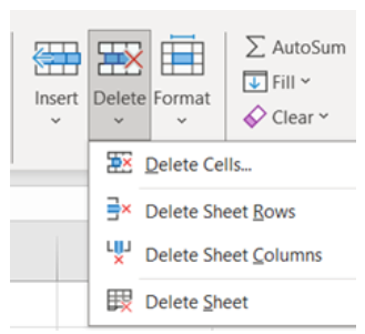
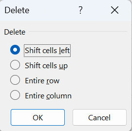
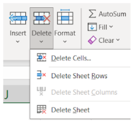
- For more options when deleting cells, select the down arrow to the right of the Delete command in the Cells group. The options provided allow the user to delete the cells, rows, columns, or the worksheet (Figure 10A). If Delete Cells… is selected, the Delete dialog box opens, providing additional options (Figure 10B).
- A cell or multiple cells can be deleted by using the delete option on the right click menu. To use, right click on the cell(s) and select Delete. The Delete dialog box opens providing additional options (Figure 10B).
- The Delete dialog box can also be opened by using the keyboard shortcut keys (Ctrl + – [minus sign]).
To insert a cell or cells: Select the cell. Click the Insert command in the Cells group on the Home tab. A new cell will be added above the selected cell.
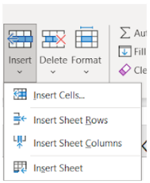
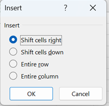
- For more options when adding cells, select the down arrow to the right of the Insert command in the Cells group. The options provided allow the user to insert cells, rows, columns, or a worksheet (Figure 10C). If Insert Cells is selected, the Insert dialog box opens, providing additional options (Figure 10D).
- A cell or multiple cells can be inserted by using the insert option on the right click menu. To use, right click on the cell(s) and select Insert. The Insert dialog box opens providing additional options (Figure 10D).
- The Insert dialog box can also be opened by using the keyboard shortcut keys (Ctrl + Shift + plus sign [+]).
Insert, Delete, and Move Columns
When working in a worksheet, the user can insert, delete, and move columns.
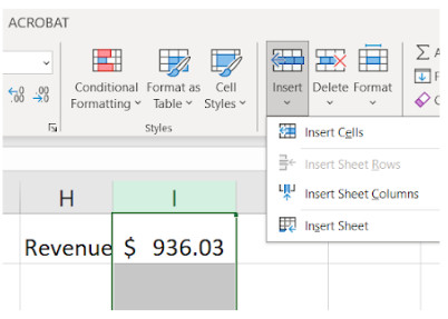
To insert a new column: Select the column heading to the right of where the new column should be inserted. (In Figure 11A, the new column will be between H and I. The I column heading must be selected.) On the Home tab, click the Insert command in the Cell group. (If the down arrow below the Insert command is clicked, a dropdown menu opens. The Insert dropdown menu also has an option, Insert Sheet Columns, which can also be used to insert a column [Figure 11A]).
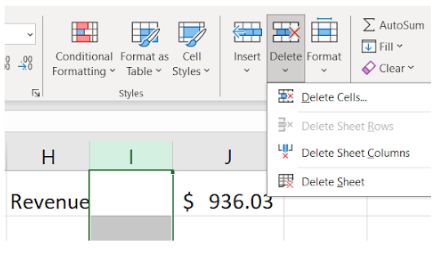
To delete a column: Select the column heading that needs to be deleted. On the Home tab, click the Delete command in the Cell group. (If the down arrow below the Delete command is clicked, a dropdown menu opens. The Delete dropdown menu also has an option, Delete Sheet Columns, which can also be used to delete a column [Figure 11B]).
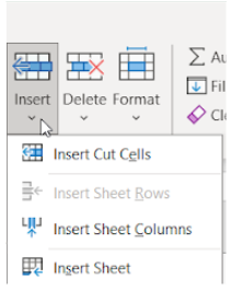
To move a column: Select the column heading of the column to be moved. Select the Cut command found on the Home tab in the Clipboard group or on the right click menu or use the shortcut keys (Ctrl + X). A dashed line border will appear around the column to be moved. Select the column heading to the right of where the column will be moved. On the Home tab, click the Insert command dropdown arrow in the Cells group. When the Insert command dropdown menu appears, select Insert Cut Cells (Figure 11C).
Insert, Delete, and Move Rows
Just like with columns, rows can be inserted, deleted, and moved in a worksheet.
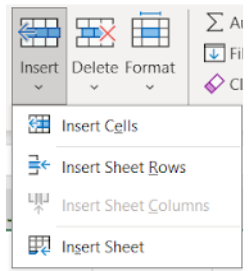
To insert a new row: When inserting a row into a worksheet, the user must select the row heading below where the new row should be inserted. On the Home tab, click the Insert command in the Cell group. (If the down arrow below the Insert command is clicked, a dropdown menu opens. The Insert dropdown menu also has an option, Insert Sheet Rows, which can also be used to insert a row. See Figure 12A).
To delete a row: Select the row heading that needs to be deleted. On the Home tab, click the Delete command in the Cell group. (If the down arrow below the Delete command is clicked, a dropdown menu opens. The Delete dropdown menu also had an option, Delete Sheet Rows, which can also be used to delete a row. See Figure 12B.)
To move a row: Select the row heading of the row to be moved. Select the Cut command found on the Home tab in the Clipboard group or on the right click menu or use the shortcut keys (Ctrl + X). A dashed line border will appear around the row to be moved. Select the row heading below the desired location of where the row will be moved. On the Home tab, click the Insert command in the Cells group. Select Insert Cut Cells from the dropdown menu.
Hide and Unhide Columns and Rows
Excel contains a tool to hide columns and rows, so they are no longer visible. Another tool allows the user to unhide the columns or rows, so they become visible again.
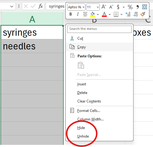
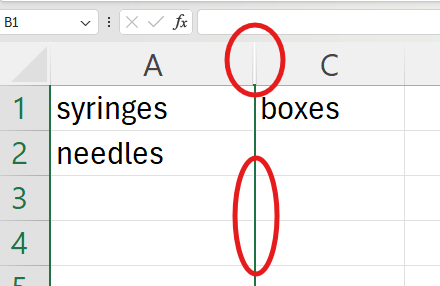
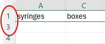
To hide columns or rows: Select the columns or rows. Right click and select Hide from the menu (Figure 13A). The columns or rows will disappear, and a line will appear in the location of the hidden column(s) or row(s) (Figure 13B). When rows and columns are hidden, the row and column headings are absent (Figure 13C).
To unhide columns or rows: Select the columns or rows on both sides of the hidden column(s) or row(s). Right click and select Unhide. The hidden column(s) or row(s) will reappear.
Merging Cells and Unmerge a Cell
Merging cells means multiple cells are used to create one cell. Merging options available in Excel are as follows:
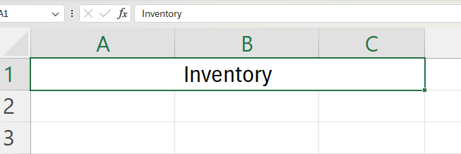
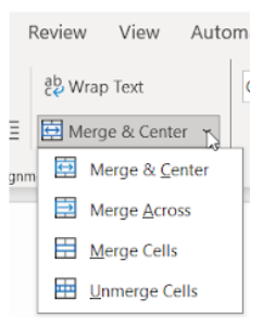
- Merge & Center: The cells selected are merged and the text is centered in the newly cell created (Figure 14A). The Merge & Center command is found in the Alignment group on the Home tab and also on the Merge & Center dropdown menu.
- Merge Across: The cells selected are merged, yet the rows are separated (Figure 14B).
- Merge Cells: The cells selected are merged into one cell. If text is present, it is not centered.
To merge cells: Select the cells to be merged. Click the Home tab and select Merge & Center command in the Alignment group (Figure 14C). Select the Merge & Center command or click the down arrow to open the dropdown menu and select from Merge & Center, Merge Across, or Merge Cells. The cells selected will become one cell (Figure 14D).
To unmerge a cell: Select the cell. Click the Home tab and select Merge & Center command in the Alignment group (Figure 14C). Select Unmerge Cells.


Learning Activities
Introduction to Excel – Flash Cards
Application Exercise 1
Directions: Create and modify a worksheet.
1. Open a new Excel workbook and save as: Exercise 12 1
2. Create the worksheet shown in Figure 15A.
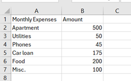
3. Adjust the column width as needed to see the text.
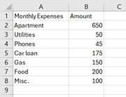
4. Insert a row below Row 5 and add Gas in Column A and 150 in Column B.
5. Change the Amount for the Apartment to 650.
6. Save the workbook. Your worksheet should look like Figure 15A.
A spreadsheet program file created in MS Excel. Contains one or more worksheets.
Found within a workbook; also called a spreadsheet. Consists of cells that can contain data, formulas, and functions.
Any of two or more vertical sections of type on a document.
The horizontal series of cells separated by lines or space form other horizontal series of cells and found in a table or spreadsheet.
A predefined formula in a spreadsheet that performs a calculation with specific values.
A mathematical equation in a spreadsheet that performs a calculation and shows the result in a cell.
A unique name or address of cell that is based on a set of coordinates that a cell occupies on a worksheet. For example, a cell that appears in Column C and in Row 8 is C8.
Also called row header. The shaded area at the left side of each row. By clicking the row header, the user selects the entire row. The row height can be changed by dragging the line below the row heading.
Also known as column headers. The shaded area at the top of the column and contains a letter or a series of letters (e.g., XA, BB). By clicking the column header, the user selects the entire column. The column width can be changed by dragging the line to the right of the heading.
Close to or next to.
A tool indicated by a plus sign cursor that is observed when the user moves the cursor to the bottom right corner of a selected cell or cell range in Excel. This tool is used to fill or extend a series or data.
Moving the mouse pointer over an option without selecting it.
To highlight a cell or multiple cells (cell range) and the next command will impact these cells.

