Chapter 13 Formatting in Excel
Vocabulary
Cell: A single box on a table or spreadsheet that can contain text (e.g., letters, numbers, dates).
Collated: Assembled in a specific way.
Column: The vertical series of cells separated by lines or space from other vertical series of cells and found in a table or spreadsheet.
Dialog box launcher: A button (with a picture of an arrow) found on the lower right corner of Ribbon groups that is used to open the dialog box.
Formula: A mathematical equation in a spreadsheet that performs a calculation and shows the result in a cell.
Landscape orientation: The orientation of the page is such that the top and bottom are longer than the sides.
Portrait orientation: The orientation of the page is such that the sides are longer than top and bottom.
Row: The horizontal series of cells separated by lines or space form other horizontal series of cells and found in a table or spreadsheet.
Workbook: A spreadsheet program file created in MS Excel. Contains one or more worksheets.
Worksheet: Found within a workbook; also called a spreadsheet. Consists of cells that can contain data, formulas, and functions.
Introduction
Excel has many formatting features that allow the user to create professional-looking spreadsheets. This chapter focuses on formatting font and numbers and creating borders. Tools such as Format Painter, Spell Check, and Find and Replace are also discussed and are similar to MS Word. The chapter concludes with a discussion on printing worksheets.
Formatting and Editing Cells
Many of the formatting and editing tools in Excel are similar to those in Word. A couple are unique to Excel. This section discusses tools used to format and edit cells, including formatting text and numbers, centering across selecting, wrapping text, aligning items, using spell check, and using find and replace.
Formatting Font
Just like in Word, the font in Excel can be formatted. The size, type, and color can be modified. Text can be bold, italicized, or underlined. These formatting commands are located on the Home tab in the Font group (Figure 1A).
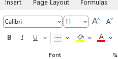
To format text, the first step includes selecting the cell(s). Then, use the following commands, found in the Font group on the Home tab:
- To change the font type: Click into the text box and type the font type or use the down arrow and select an option. By default, the font used in workbooks is Calibri.
- To change the font size: Click into the text box and type the font size or use the down arrow and select an option.
- To increase the font size: Click on the Increase Font Size command to the right of the font size box.
- To decrease the font size: Click on the Decrease Font Size command to the right of the Increase Font Size command.
- To bold the font: Click the Bold command found under the Font box. The keyboard shortcut keys (Ctrl + B) can also be used.
- To italicize the font: Click the Italic command to the right of the Bold command. The keyboard shortcut keys (Ctrl + I [capital I]) can be used.
- To underline the font: Click the Underline command to the right of the Italic command. The keyboard shortcut keys (Ctrl + U) can be used.
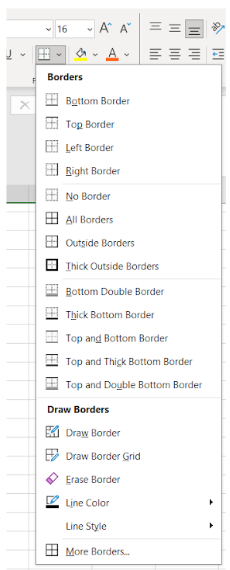
- To add borders to the cell(s): Click the Borders command or the down arrow to the right of the command, which opens the Borders menu (Figure 1B). Select the desired option on the menu, and the border(s) is applied to the cell(s). (Additional information on borders will be discussed later in the chapter.)
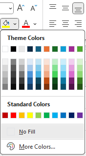
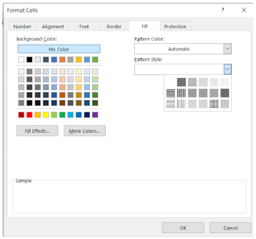
- To add background color to the cell(s): Click the Fill Color command or the down arrow to the right of the command, which provides additional background colors (Figure 2A). To remove fill, select No Fill. For additional colors, select More Colors, which is similar to Word.
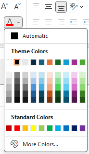
- To change the font color: Click the Font Color command or the down arrow to the right of the command to open a menu of additional font color options (Figure 2B).
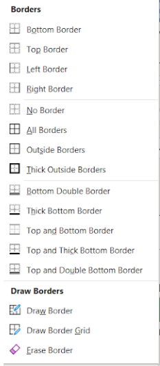
Figure 1B. Borders Dropdown menu.
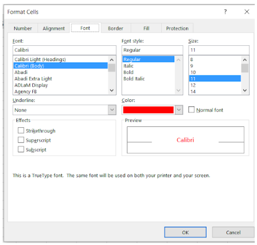
Formatting text options is also available using the right click menu after a cell is selected (Figure 2C). Additional formatting options are available using the dialog box launcher in the Font group. The Font, Border, and Fill tabs can be used to apply the formatting discussed above (Figures 2D and 2E).

Formatting Numbers
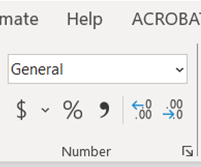
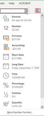
In Excel, the user can format numbers in a variety of ways, including currency, date, time, decimals, and percentages (see Table 1 below). The commands in the Number group in the Home tab can be used to apply number formatting to a cell or cell range (Figure 3A).
Additional formatting options are available by clicking the down arrow to the right of the Number Format box. When this is done, a dropdown menu with additional formatting options appears (Figure 3B). Several formatting commands are available below the Number Format box, including accounting number format, percent and comma styles, and increase and decrease decimals.
| Format | Description |
|---|---|
| General | Default style; the number is shown how it is typed. |
| Number | Can be used for numbers with decimal places. The number of decimal places, the format for negative numbers, or the use of the Comma Style can be determined by the user. |
| Currency | Used to show a monetary amount. The dollar sign is next to the first digit. The number of digits after the decimal point can be determined by the user. |
| Accounting | Similar to the currency format with the exception of the left margin alignment of the dollar sign and the alignment of the decimal point. |
| Date | Long and short date options are available. Long date would include the month, day, and year written out (e.g., Monday, October 9, 2023). A short date includes a two-digit month and day and a four-digit year (e.g., 10/09/2023). Date formats that have an asterisk (*) change with the regional date settings in the Control Panel. |
| Time | Displays in a time format. Several time formats are available, along with some with the date. Time formats that have an asterisk (*) change with the regional time settings in the Control Panel. |
| Percentage | The number is displayed with a percent sign. The number of digits after the decimal can be set. |
| Fraction | Numbers can be displayed as fractions. |
| Special | Numbers can be displayed as ZIP code, Social Security number, and phone number. |
Using the Format Cell Dialog Box
Number formatting options are also available by selecting the dialog box launcher in the Number group or by selecting More Number Format on the Number Format dropdown menu (Figure 3C). This opens the Format Cell dialog box on the Number tab page. Select the category on the left side of the dialog box. Additional options for the category are available on the right side of the dialog box. Once the selections are made, click OK. The desired formatting is applied to the cell or cell range.
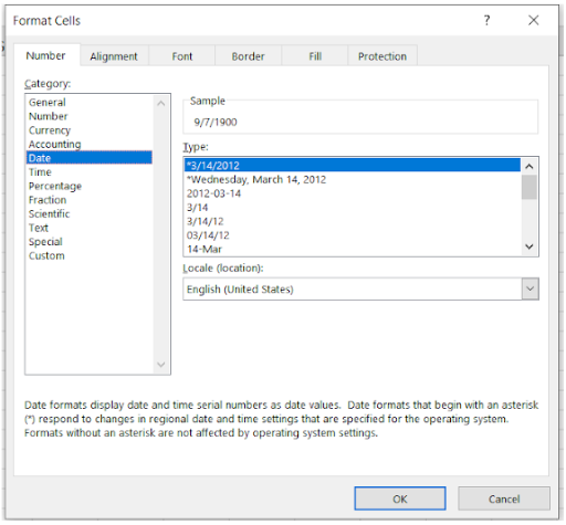
Number formatting can also be done by selecting a cell or cell range and right clicking. Select Format Cell on the menu. This action opens the Format Cell dialog box described above.
Keyboard Shortcuts
Keyboard shortcut keys and other shortcuts can also be used to add formatted numbers to a worksheet:
- To add the current time to a cell: Use (Ctrl + Shift + : [colon key]).
- To add the current date to a cell: Use (Ctrl + ; [semicolon key]).
- To apply the currency format to a cell or cell range: Use (Ctrl + Shift + $ [dollar sign key]). Also, by just typing a $ before a number (e.g., $12.36), it applies the currency format to the cell.
- To apply the percentage format to a cell or cell range: Use (Ctrl + Shift + % [percent sign key]). Also, just by adding % after a number (e.g., 35%), it applies the percentage format to the cell.
- To apply the scientific number format with two decimal places: Use (Ctrl + Shift + ^ [caret sign key]).
To format a cell or multiple cells using the Number group commands: Select the cell or cell range. Select the desired option listed in the Number group on the Home tab or on the Number Format dropdown menu. If needed, add a comma by selecting the Comma Style command and adjust the numbers to the right of the decimal point using the Increase Decimal or Decrease Decimal commands.
Using Center Across Selection
The Center Across Selection will center the text across the selected cells, but the cells are not merged. This can be beneficial if the user needs to manipulate the worksheet later.
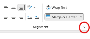
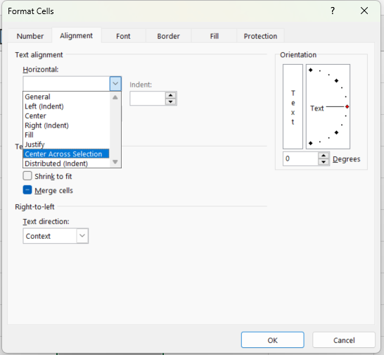
To use the Center Across Selection: Select the cells to be used. Click the dialog box launcher in the lower right corner of the Alignment group on the Home tab (Figure 4A). The Format Cells dialog box will open. On the Alignment tab, under the Text alignment, click the down arrow to open the Horizontal dropdown menu. Select Center Across Selection (Figure 4B). The cells will appear as they are merged, but each cell is retained and has a unique address (Figure 4C).

Wrapping Content in a Cell
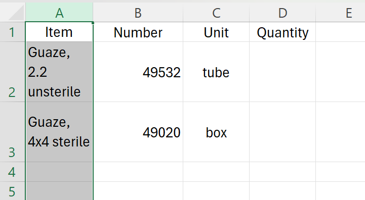
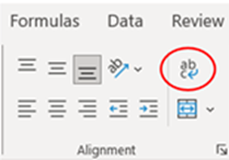
When there is too much content in a cell, only part of it will show (Figure 5A). If the user wants all of the content to show, the Wrapping Content command can be used. The content will appear in multiple rows within the cell, and the row height will be increased in size (Figure 5B).
To wrap text: Select the cell. Click the Home tab and select the Text Wrap command in the Alignment group (Figure 5C). The text is then wrapped in the cell.

Aligning and Orienting Text
Alignment can be applied to one cell, a cell range, row(s), column(s), or the entire worksheet. (To select all cells, the keyboard shortcut keys (Ctrl + A) can be used.
Horizontal and Vertical Alignment
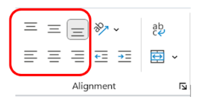
When text is aligned, it is positioned in a specific location in the cell. Text can be vertically aligned in the top, middle, or bottom of the cell. Middle alignment centers the text with equal distance from the top and bottom of the cell. Text can also be horizontally aligned on the left, center, or right side of the cell. Center alignments position the text in the middle of the cell, so there is equal distance on the right and left side.
To apply alignment to a cell or multiple cells: Select the cell(s) to be aligned. On the Home tab, in the Alignment group, select the horizontal and/or vertical alignment option desired (Figure 6).
Orientation Command
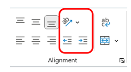
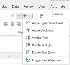
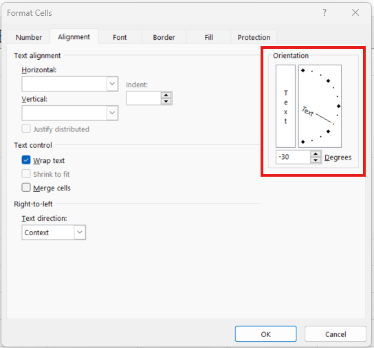
The Orientation command can be used to rotate the text in the cell (Figure 7A). Text can be rotated counterclockwise, clockwise, vertical, up, and down (Figure 7B). The Format Cell Alignment option on the Orientation command menu opens the Alignment tab on the Format Cell dialog box. Additional options for orientation are available by using the options in this dialog box, including setting a specific text orientation degree.
To rotate text: Select the cell(s), row(s), column(s), or cell range. Click the Orientation command found in the Alignment group on the Home tab. Select the desired option from the Orientation command menu. If the Format Cell Alignment option is selected, the Format Cells dialog box opens. To change the text orientation, the user can either type the degrees in the text box, use the up or down arrows, or drag the line after Text in the orientation box to the desired location. (See the arrow in Figure 7C.) When dragging the line, the orientation degrees appear in the text box. When the desired orientation is achieved, click OK.
Decrease and Increase Indent Commands
The Decrease Indent command moves text in the cell to the left margin. The Increase Indent command moves the text in the cell to the right margin. These commands can be applied to one or more cells, rows, or columns.
To use the Decrease Indent and Increase Indent commands: Select the cell(s) to be aligned. On the Home tab, in the Alignment group, select either the Decrease Indent command or the Increase Indent command (Figure 7A). Press the key until the text is in the desired location.
Adding Borders
Predefined cell borders and custom borders can be added to cells or cell ranges in a worksheet.
To apply a predefined cell border: Select the cell or cell range that will have the border. Click the arrow to the right of the Border command in the Font group on the Home tab. When the Border command menu opens, select a border style in the Border section (Figure 8A). The border will be applied to the cell or cell range selected.
To change the color and/or line style: Select the cell or cell range. Click the arrow to the right of the Border command in the Font group on the Home tab. Select Line Color or Line Style on the menu and then the desired color or style. The pointer will change to a pencil icon (Figure 8B). Click the cell border(s) to add the border. The same line color and style will be applied until another color or style is selected. To change the color or style, click on the arrow to the right of the Border command. Select Line Color or Line Style and select the desired options. Click the cell borders to apply the new borders. Press the ESC key to turn off/stop applying the borders.
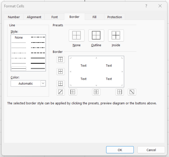
Apply customized borders: Select the cell or cell range that will have the border. Click the arrow to the right of the Border command in the Font group on the Home tab. When the Border command menu opens, select More Borders at the bottom of the menu (Figure 8A). The Format Cell dialog box will open (Figure 8C). On the Border tab, start by selecting the line style and color on the left side of the box. Then, either select a preset border or click the individual border buttons, and the border will appear in the box. If a second border color and/or line style must be added to the same cell or cell range, select the new style and/or color on the left side of the dialog box. Select the preset border or the individual border buttons. When the border selection is completed, click OK.

To remove a border: One of these two options can be used:
- Select the cell or cell range where the border needs to be removed. On the Home tab, click the arrow to the right of the Border command. Select No Border.
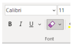
- On the Home tab, click the arrow to the right of the Border command. Select Erase Border. The pointer will appear as an eraser (Figure 9A), and the button will turn gray (Figure 9B). Click on each cell border that needs to be removed. Click the Erase Border button to stop erasing borders.

Using Gridlines
The gridlines are faint lines that border cells. By default, gridlines are visual to the user on the monitor, but not when the workbook is printed. Gridlines can be removed or shown for the entire worksheet. The colors of the gridlines can also be changed.
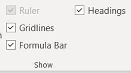
To remove gridlines: Using the View tab, remove the checkmark to the left of Gridlines in the Show group (Figure 10A).
To add gridlines: Using the View tab, click the box (to add the checkmark) to the left of Gridlines in the Show group.
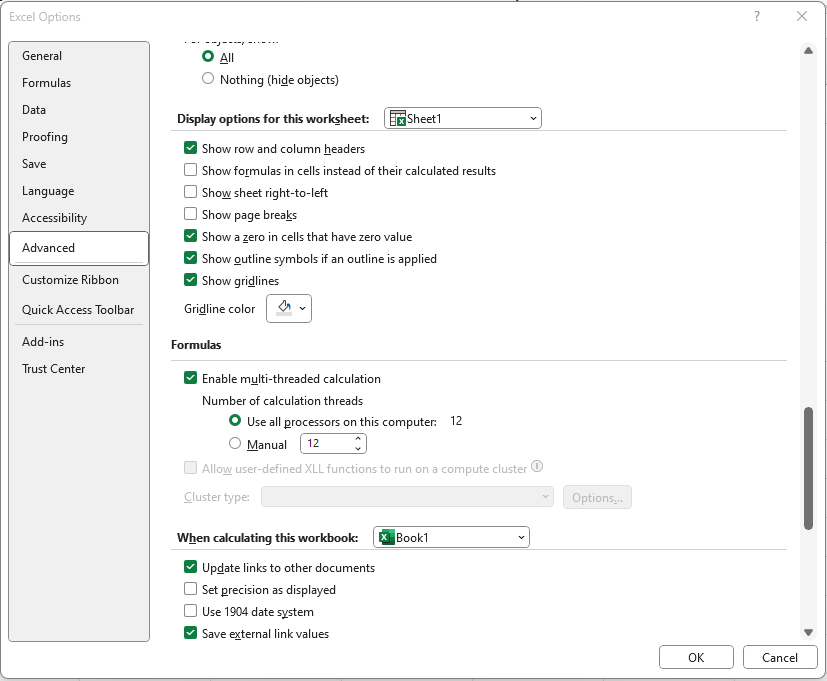
To change the gridline color: Using the File tab, click Options. On the Excel Options dialog box, select Advance and scroll to the Gridline color option (Figure 10B). Click the down arrow to the right of the pail icon. Select a color and click OK. The worksheet gridline colors changes to the new selected color.
Using the Format Painter
The Format Painter can quickly apply the formatting of one cell to other cells. Formatting can include the text type, color, size, alignment, and number formatting. All the formatting applied in the initial cell can be copied using the Format Painter and applied to other cells.
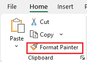
To use the Format Painter: Select the cell with the formatted text. On the Home tab, click the Format Painter command in the Clipboard group (Figure 11A). The pointer will turn to a paint brush (Figure 11B). To apply the format to a cell, click on the cell. To apply the format to a complete row or column, click on the row heading or column heading.
A single click on the Format Painter command will allow the format to be applied to one cell, column, or row. To apply formatting to multiple locations, double-click the Format Painter command. The button will remain on, allowing formatting to be applied to multiple cells, columns, and/or rows until the command is clicked again. When Format Painter command is on, the gray box will appear behind the paint brush icon on the button (Figure 11A).

Using Spell Check
The contents of the worksheet can be spell checked. Spelling can be checked in selected cell(s), rows, or columns. The Spelling command can be found on the Quick Access Toolbar or on the Review Tab in the Proofing group.
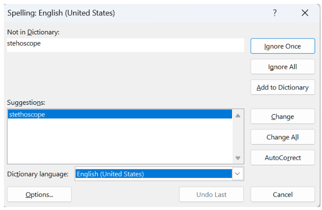
To check the spelling of cell(s): Select the cells, rows, or columns to be checked. Click on the Spelling command found in the Proofing group on the Review tab. If a spelling error exist, the Spelling dialog box appears (Figure 12). Possible words appear in the Suggestions box. The user can select to ignore it once or always. The user can select the correct word and then click Change or Change All (occurrences of the word in the selected cells).
Using Find and Replace
The Find command allows the user to locate specific text or a number in the worksheet. The Find and Replace command allows the user to find and revise content.
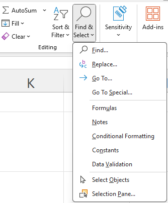
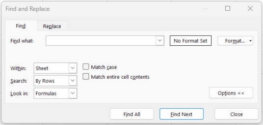
To find specific content: On the Home tab, select Find & Select command in the Editing group. When the dropdown menu opens, select Find (Figure 13A). The Find and Replace dialog box opens. On the Find tab, type the content to find. Additional options are available when the Options button is selected (Figure 13B). The user can either see one or all instances of the word/phrase:
- To see one instance at a time, click Find Next. The tool will find the next instance of the word, phrase, or number in the Find box. Continue to use Find Next to move through the worksheet.
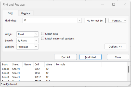
- To see all of the instances at once, click Find All. A box at the bottom of the dialog box will open a listing of all instances of the text or number (Figure 13C).
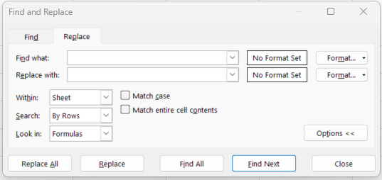
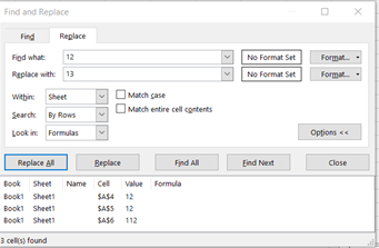
To find and replace specific content: On the Home tab, select Find & Select command in the Editing group. When the dropdown menu opens, select Find. The Find and Replace dialog box opens. On the Find tab, type the content to find and click Replace (Figure 13A). On the Replace tab in the Find and Replace dialog box, type the word, number, or phrase to find and the text or number to replace it with. Additional options are available when the Options button is selected (Figure 13D). The user can replace the text or number individually or all at once following these steps:
- To replace the content individually, select Find Next and then Replace. Continue this process until the worksheet is completed.
- To replace the content at once, select Find All. A box will appear at the bottom of the dialog showing each instance of the content in the worksheet and indicate the location (Figure 13E). Select Replace All to replace all the content at once. When all replacements are made, a message will appear indicating the number of replacements completed. Select OK.
Working With Multiple Worksheets
By default, when a new workbook opens, the worksheet is called “Sheet1.” Each time the user clicks the plus sign to the right of the workbook tabs, a new worksheet is added to the workbook. Figure 14A shows four worksheets added to the workbook. The default name of the worksheets is “Sheet” followed by a number.
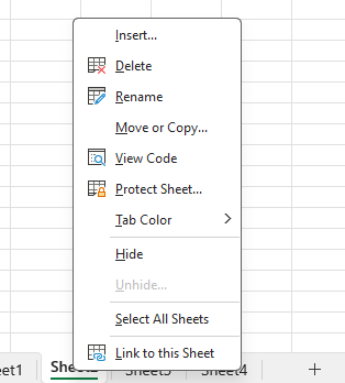
Clicking on the worksheet tab will make that worksheet active. Right clicking on the tab will open a menu (Figure 14B). Many commands are available on the menu to the user, including the following:
- Delete: Select to delete the worksheet from the workbook.
- Rename: Select to rename the title of the worksheet. To rename the tab, right click on the tab and select Rename. When the current tab name is highlighted, type the new name (Figure 14C) and press the Enter key.
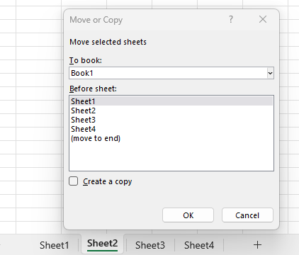
- Move or Copy: When selected, the Move or Copy dialog box opens (Figure 14D). The user can move the tab to another location or copy the tab. When the copy is made, the tab name indicates the copy by having a (2) follow the tab name (Figure 14E).
- Tab Color: Allows the user to apply a color to a tab. To apply a tab color, right click on the tab and select Tab Color. Select the desired color.
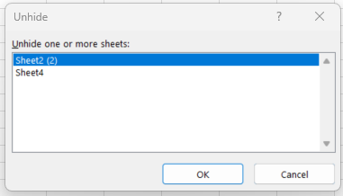
- Hide: Allows the user to hide the selected tab. Once a tab or tabs are hidden, “Unhide…” appears below “Hide” on the right click menu. To make a hidden tab visible, select Unhide on the menu. On the Unhide dialog box, select the tab name to make visible and then select OK (Figure 14F).



Using the File Tab
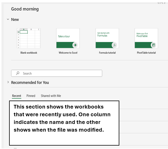
When the user clicks the File tab, the Backstage view opens. The options available to the user are similar to those in Microsoft Word and some of these include the following (Figure 15):
-
- Back arrow (indicated by a circled arrow): The user can click the arrow to close the Backstage view and return to the worksheet.
- New: To open a new workbook or template, the user can click New and then Blank workbook or another template. A template includes customized formatting and predefined formulas in the predesigned spreadsheet.
- Open: The user can open a previously saved workbook. After selecting Open, the user can select Computer and then click Browse. When the Open dialog box appears, the user can navigate to find the saved workbook. Select the workbook and then click Open on the dialog box.
- Info: This provides information on the currently opened workbook, including protection options, version history, and inspecting the workbook for issues.
- Save: This command is used to save the workbook after changes are made. The first time a workbook is saved, the user will need to choose the location, a file name, and the file type. The saving process is similar to the process described in the Word chapter.
- AutoRecover: By default, Excel autosaves the workbook every ten minutes. If the workbook is not saved before it is closed, the user can restore the file using AutoRecover. When the workbook is reopened, the Document Recovery pane will reappear if autosaved versions are available. The user can click the autosaved version to recover the workbook.
- Save As: This command allows the user to save a copy of the workbook or to save the workbook onto another drive.
- Print: This allows provides the user with options for printing the worksheet.
- Share: The user can invite others to view the spreadsheet or email the spreadsheet as an attachment.
- Export: The user can export the workbook into an Adobe Acrobat document (also known as a PDF file). After selecting Export, click Create PDF/XPS and complete the fields in the Save As dialog box. Click Publish. By default Excel exports only the active worksheet.
- Options: Provides options to the user that relate to language, proofing, data, and formulas.
Printing a Section of the Workbook
The entire workbook can be printed or just a selected area.
Setting and Clearing Print Areas
The user can also select just a specific section of the workbook to print. To do this, the user must define a print area. The print area is a range of cells that are selected to be printed. A workbook can have multiple print areas, and each will print on a separate page.
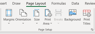
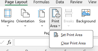
To select a specific print area(s): Select the cells for the print area. Using the Page Layout tab, click Print Area in the Page Setup group (Figure 16A). Then, click Set Print Area on the menu. To set multiple print areas, press and hold the Ctrl key while clicking the areas to print.
To add adjacent cells to an existing print area: Select the adjacent cells next to the existing print area. Using the Page Layout tab, select the Print Area command in the Page Setup group. Select Add to Print Area on the menu (Figure 16B).
To clear the print area(s) on a worksheet: Select a cell in the worksheet. Using the Page Layout tab, select the Print Area command in the Page Setup group. Select Clear Print Area on the menu (Figure 16B).
Print a Worksheet or a Print Area
To print, select the File tab. Click Print. Use the arrows and dropdown menus to select the desired options.
- Copies: Indicate the number of copies desired.
- Printer: Select the printer.
- Settings:
- Select the area to print.
- Select to print either on one side or both sides.
- Select collated (1,2,3; 1, 2, 3) or uncollated (1,1,1; 2,2,2).
- Select the orientation. By default, portrait orientation is applied to the worksheet. The orientation can be modified to landscape orientation by either on the Print screen or by using the Page Layout tab and clicking the Print Area in the Page Setup group (Figure 16A).
- Select the paper size.
- Select the margins.
- Select no scaling (print sheets in the actual size) or scaled options to include the entire worksheet on one page or fit all columns or rows on one page.
Learning Activities
Formatting in Excel – Flash Cards
Application Exercise 1
Directions: Create a worksheet and format the content.
- Open a new Excel workbook and save as: Exercise 13 1
- Create the worksheet shown in Figure 17A.
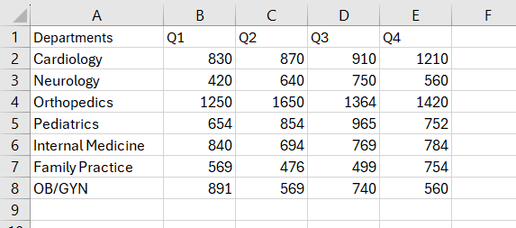
Figure 17A. Practice worksheet. - Adjust the column width as needed to see the text.
- Insert two rows above the current Row 1. (Departments should now be in Row 3.)
- Format the text in the cell range A4:A10 by using Arial 11 pt italic font.
- Format the font in Row 3 by using Arial 12 pt bold font and center font.
- Format the font in the cell range B4:E10 by using Arial 11 pt.
- Apply the Accounting format to the cell range B4:E10. Do not have any decimals and use the dollar sign ($).
- Using the cell range A1:E1, apply Center Across Selection and add the title: Quarterly Expenses
- Format the font in Row 1 by using Arial 14 pt bold font in a blue shade of your choice.
- Apply borders to the cell range A3:E10. Apply a blue border, using a style and blue shade of your choice.
- Rename the worksheet tab to: Expenses.
- Apply a blue shade to the worksheet tab.
- Save the workbook. Your worksheet should look like Figure 17B.
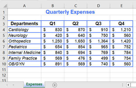
Figure 17B. Completed practice worksheet.
Found within a workbook; also called a spreadsheet. Consists of cells that can contain data, formulas, and functions.
A single box on a table or spreadsheet that can contain text or numbers.
A button (with a picture of an arrow) found on the lower right corner of Ribbon groups that is used to open the dialog box.
The horizontal series of cells separated by lines or space form other horizontal series of cells and found in a table or spreadsheet.
Any of two or more vertical sections of type on a document.
A spreadsheet program file created in MS Excel. Contains one or more worksheets.
A mathematical equation in a spreadsheet that performs a calculation and shows the result in a cell.
Assembled in a specific way.
The orientation of the page is such that the sides are longer than top and bottom.
The orientation of the page is such that the top and bottom are longer than the sides.

