Chapter 14 Excel Formulas, Functions, and Tables
Vocabulary
Absolute reference: The cell reference in the formula is constant (always use the same cell) even when it is copied to other cells. Is also called absolute cell reference.
Argument: The independent variable of a function.
Banded: Having strips or bands of contrasting colors.
Cell: A single box on a table or spreadsheet that can contain text or numbers.
Column: The vertical series of cells separated by lines or space from other vertical series of cells and found in a table or spreadsheet.
Formula: A mathematical equation.
Function: A predefined formula in Excel that consists of an equal sign, a function name, and an argument.
Header row: The top row of a table that contains the titles for the columns.
Hover over: Moving the mouse pointer over an option without selecting it.
Relative reference: The cell reference changes when the formula is copied to another cell; also called relative cell reference.
Row: The horizontal series of cells separated by lines or space form other horizontal series of cells and found in a table or spreadsheet.
Table: A rectangular grid consisting of columns and rows. Allows for an orderly arrangement of data.
Creating Formulas
Using formulas to perform calculations and other tasks is a powerful feature of Excel. Excel can add, subtract, multiply, and divide numbers. Numbers in cells can be used in the calculations.
Basics of Formulas
When building formulas in Excel, all formulas must begin with an equal sign (=). Table 1 shows the standard operators used in Excel. A formula can include numbers (e.g., =2*3) or cell references/cell addresses (e.g., =A1*B1) (Figure 1). After the formula is created and the user presses the Enter key, the calculation is completed, and the answer appears in the cell. With cell references, if the values in the cells change, the formula automatically recalculates and updates the answer.
| Standard Operator | Formula Example | |
|---|---|---|
| Addition | Plus sign (+) | =A1+A2 |
| Subtraction | Minus sign (-) | =A1-B1 |
| Multiplication | Asterisk (*) | =A1*B1 |
| Division | Forward slash (/) | =A1/B1 |

Using Symbols in Formulas
Several symbols are used in Excel formulas. Table 2 indicates some of the more commonly used symbols. Figures 2A and 2B show formulas that use symbols. There can be several ways to write a formula in Excel. For example, Figures 1, 2A, and 2B are three different ways to calculate the three cells. The answers are the same, but the formulas can be written differently. This chapter will cover just some of the ways to create basic formulas.
| Name | Symbol | Description | Formula Example |
|---|---|---|---|
| Equal to (equal sign) | = | Every Excel formula must start with an equal sign. | =A1+B1 |
| Parentheses | ( ) | Contain the independent variables of the function. | =MAX(A1:C1) |
| Numbers or cell references in the parentheses will be calculated first. | =A1+B1+(C1*D1) | ||
| Dollar sign | $ | Used for absolute cell reference in Excel formula. | =($A1*$B$2) |
| Colon | : | References all cells between the two cell addresses. For instance, A1:C1 includes A1, B1, and C1. | =A1:C1 |


Create Formulas
There are several ways to create basic formulas. The user can type the formula into the cell, click to select cells to be included in the argument, or copy the formula to other cells. When creating a formula, it will be visible in both the cell and also in the formula bar. The user can place the pointer in either location to create the formula.
Typing a formula in a cell: Select the cell where the formula will be entered. Type an equal sign (=). Type the cell address in the cell. Add the standard operator (e.g., +, -, *, or /). Type the cell address in the cell. Continue to add the standard operator, along with the cell address until all the cells desired are entered. Press the Enter key. The formula will calculate, and a value will be visible in the cell.
Use the point and click method to create a formula: Select the cell where the formula will be entered. Type an equal sign (=). Click the first cell to be included in the argument, and the cell address appears in the formula. Add the standard operator (e.g., +, -, *, or /). Click the next cell to be added to the argument, and the cell address appears in the formula. Continue to add cell addresses and standard operators until the desired formula is created. Press the Enter key. The formula will calculate, and a value will be visible in the cell.
Edit and View Formulas
Once a formula is created, it can be revised and viewed. The user can also cancel edits during the revision process.
To edit a formula: Select the cell with the formula to edit. Click the formula bar or double-click into the cell to edit the formula. Revise the formula as needed, and then press the Enter key on the keyboard or click the Enter command on the formula bar (Figure 3).
To cancel the edit: Click the Cancel command on the formula bar or press the ESC key on the keyboard.
To view existing formulas on the worksheet: Select the Formula tab and click Show Formula command in the Formula Auditing group. All the formulas in the worksheet become visible. To hide the formulas, click the Show Formula command again. The keyboard shortcut to show existing formulas is (Ctrl + `[grave accent mark]). To hide the formulas, press the keyboard shortcut again.

Copy Formulas
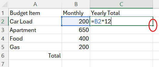
There are several ways to copy a formula to additional cells. Two common ways to copy formulas include using the fill handle and the right click menu. A formula can be copied to adjacent cells by using the fill handle (Figure 4A). The copy and paste technique using the right click menu can copy the formula to any cell on the worksheet.
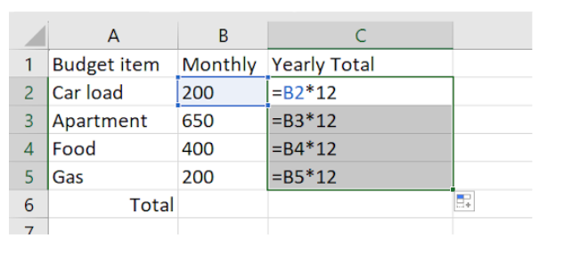
Copy the formula using the fill handle: Select the cell with the formula to copy. Click and drag the fill handle over the cells to be filled (Figure 4B). The formula will be copied to the cells when the mouse click button is released.
Copy and paste the formula: Right click on the cell with the formula to copy. Select Copy on the right click menu. Select the cells to fill with the formula. Right click and select Paste from the menu. The formula will be pasted in the selected cells.
Relative Reference
By default, Excel adjusts the cell address for each additional line when a formula is copied. This is helpful if the same formula needs to be applied to multiple rows or columns.
For example, in Figures 4A and 4B, the formula in C2 is copied to C3:C5. Notice that in Row 2, the formula contains B2. In Row 3, the formula contains B3 and so on. The row number after the Column B changes based on the row. The changing of the cell address is known as relative reference. This is the default setting in Excel.
Absolute Reference
In the prior section, relative reference was explained. The cell reference changes when the user copies the formula to another cell. There are times when the user wants to use a specific cell reference in a formula even as it is copied to other cells. This type of cell reference is called absolute reference. When a specific row and/or column is needed in the formula even when it is copied to other cells, the absolute cell reference should be used.
To create an absolute reference, a dollar sign ($) is added before the column letter and/or row number. Table 3 describes three types of absolute references.
| Description | Format | Example |
|---|---|---|
| Column and row remain unchanged when the formula is copied. (The exact same cell will be used each time.) | Place a dollar sign ($) before the column letter and the row number. | $C$4 |
| The column remains unchanged when the formula is copied. (The row number will change.) | Place a dollar sign ($) before the column letter. | $C4 |
| The row remains unchanged when the formula is copied. (The column letter will change.) | Place a dollar sign ($) before the row number. | C$4 |
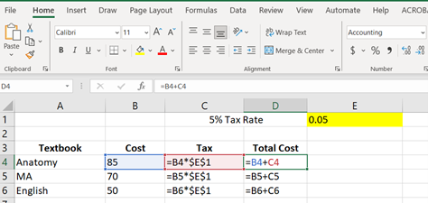
To use an absolute reference: Select the cell where the formula will be entered. Type an equal sign (=). Type the formula as described in a prior section. Determine if a column and/or row need to be constant as the formula is copied. If so, insert a dollar sign ($) before the column letter to keep the column constant and/or before the row number to keep the row constant (Figure 5). Press the Enter key. The formula will calculate, and a value will be visible in the cell. Use one of the formula-copying techniques to copy the formula to the additional cells.
Using Functions
Functions are predefined formulas in Excel. A function is created with three basic parts (Figure 6A):
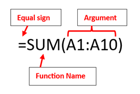
- Equal sign: All formulas (including functions) must start with an equal sign.
- Function name: The name of a predefined formula. Excel contains hundreds of functions, which are divided into several subcategories, such as Text, Financial, and AutoSum. The Formula tab contains a Function Library group (Figure 6B). Table 4 provides a list of some of the more common function names.

Figure 6B. The Function Library on the Formula tab.
- Argument: Refers to both specific cells and cell ranges, which are enclosed in parentheses. A function may have one argument like the examples in Table 4. Functions may also have multiple arguments, which are separated by a comma. An example of a multiple argument function would be the following: =sum(C1:C4, D3:D6, F1).
| Function Name | Description | Formula Example |
|---|---|---|
| SUM | Adds the values of the cells. | =SUM(A1:A4) |
| AVERAGE | Finds the average. | =AVERAGE(A1:C1) |
| COUNT | Counts the number of cells that contain numbers. (A cell with a zero is counted.) | =COUNT(A1:C1) |
| COUNTA | Counts the number of cells that contain numbers, letters, and spaces. | =COUNTA(A1:C1) |
| MAX | Used to find the largest number in the cell range. | =MAX(A1:C1) |
| MIN | Used to find the smallest number in the cell range. | =MIN(A1:C1) |
Add a function to a cell: Select the cell where the function will be added. Type the equal sign and function name. Type a parenthesis, cell reference (cell range), and a parenthesis. Press the Enter key. For example, if all cells with numbers, spaces, and text need to be counted for A1:Z1, the function would be as follows: =COUNTA(A1:Z1)
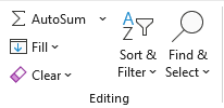
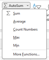
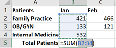
Add a function using the AutoSum command: Select the cell where the function will be added. On the Home tab, select the AutoSum command in the Editing group or use the keyboard shortcut (ALT + = [equal key]), if summing the cell range is required (Figure 6C). Otherwise, click the down arrow to the right of the command to open the dropdown menu (Figure 6D). Select the desired function name. The function is inserted into the cell, and the cells in the argument are highlighted (Figures 7A and 7B). If the selected cells need to be modified, click and drag the mouse to select the correct cells for the argument or manually enter the cell range into the argument. Once the correct cells are highlighted, press the Enter key, and the calculation will be performed and the value shown.

Copying functions to adjacent cells: Select the cell with the function. Click and drag the fill handle over the cells to be filled.
Special Viewing Options
As a worksheet grows in size, viewing the data can become more difficult. Excel has embedded tools to assist the user with this challenge. Freezing one or more rows or columns helps the user view data while moving through a large worksheet. The worksheet can also be split into panes to assist with viewing. A new window with a worksheet from the workbook can also be added.
Freeze Rows or Columns
When working with large worksheets, seeing certain rows and columns can be helpful. Excel has a tool that allows the user to freeze a row or a column.
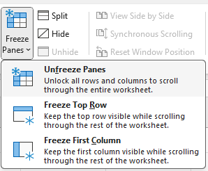
To freeze the top row: Using the View tab, select the Freeze Pane command in the Windows group (Figure 8A). When the dropdown menu appears, select Freeze Top Row (Figure 8B).

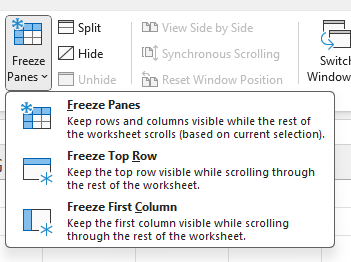
To freeze the first column: Using the View tab, select the Freeze Pane command in the Windows group. When the dropdown menu appears, select Freeze First Column.
To freeze a row(s): Select the row below the row(s) to be frozen. Using the View tab, select the Freeze Pane command in the Windows group. When the dropdown menu appears, select Freeze Pane. The rows above the selected row will remain visible. A gray line will be on the bottom border of the frozen rows. For example, in Figure 8C, Row 3 and Freeze Pane were selected on the dropdown menu. Thus, Rows 1 and 2 are now always visible on the worksheet above the gray line.

To freeze a column(s): Select the column to the right of the column(s) to be frozen. Using the View tab, select the Freeze Pane command in the Windows group. When the dropdown menu appears, select Freeze Pane. The columns to the left of the selected column will remain visible. A gray line will appear on the right border of the frozen column(s). For example, in Figure 8D, Column C was selected, and Freeze Pane was selected on the dropdown menu. Thus, Columns A and B are now always visible on the worksheet followed by a gray line.
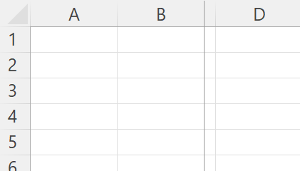
To unfreeze a panel, row, or column: Using the View tab, select the Freeze Pane command in the Windows group. When the dropdown menu appears, select Unfreeze Panes (Figure 8E).
Splitting a Worksheet
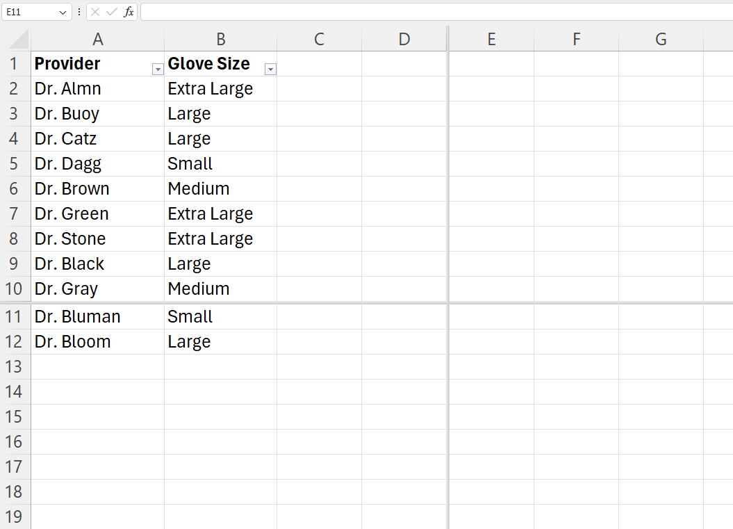
Excel contains a Split command. This allows the user to divide the worksheet into different panes, either in four panes, two vertical panes, or two horizontal panes. Depending on the selected cell, the software will split the worksheet differently.
To split the worksheet, follow these steps:
- Select a cell:
- To split a worksheet into four equal panes: Select cell A1 (Figure 9A).
- To split a worksheet into two vertical panes: Select any cell in Row 1 except cell A1. The split will appear to the left of the selected cell. See Figure 9B.
- To split a worksheet into two horizontal panes: Select any cell in Column A except cell A1. The split will appear above the selected cell. See Figure 9C.
- To split a worksheet into four panes: Select any cell other than cells in Row 1 and Column A. The selected cell will be the first cell in the bottom right pane (Figure 9D).
- Using the View tab, select the Split command in the Windows group. The split will occur.
-
- To modify the split: Click the split line in the row or column headers and drag the line to the desired location.
- To remove the split: Use the View tab and select the Split command in the Windows group.
Opening New Window(s)
The user can open additional windows for the same workbook. This allows the user to work on two different worksheets of the same workbook at the same time.
To open additional windows: Using the View tab, select the New Window command in the Windows group. The second window of the workbook appears.
To organize multiple open windows: Use the Arrange All command in the Windows group on the View tab.
Sort and Filter Data
Excel contains tools to sort data in a worksheet. It also contains commands to filter data, so only rows with specific information will be shown on the worksheet.
Sorting Data
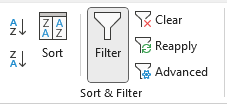
Sorting data allows the user to organize the data in the worksheet. Data can be sorted numerically (e.g., sorting zip codes) and alphabetically (e.g., sorting last names in an alphabetical order). The sort can impact the entire worksheet or just a cell range. The Sort commands are located on the Data tab in the Sort & Filter group (Figure 10A). The Sort command options are as follows:
- Sort A to Z: Organizes the data from lowest to highest.
- Sort Z to A: Organizes the data from highest to lowest.
- Sort: Selecting the Sort command will open the Sort dialog box (Figure 10B). The Sort dialog box allows the user to sort the data using one or more levels of sorts. The dropdown arrows open the menu with additional options for the sort.
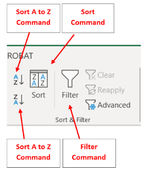
Figure 10A. The Sort & Filter group on the Data tab.
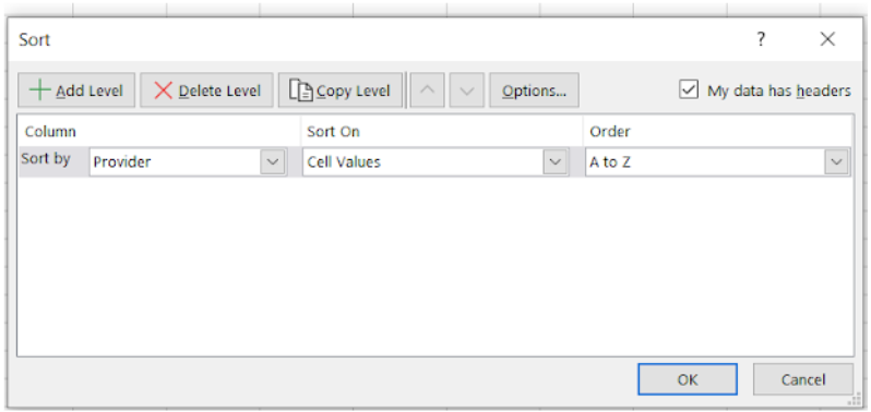
When a worksheet sort is done, information in one column is organized. The information in each row remains together when the sort is done. For instance, if a list of addresses were sorted by the cities, each person’s information remains together, though the row may move higher or lower on the worksheet.
If a sort range is done, the data in the range of cells are impacted by the sort. Content in other cells in the worksheet are not impacted.
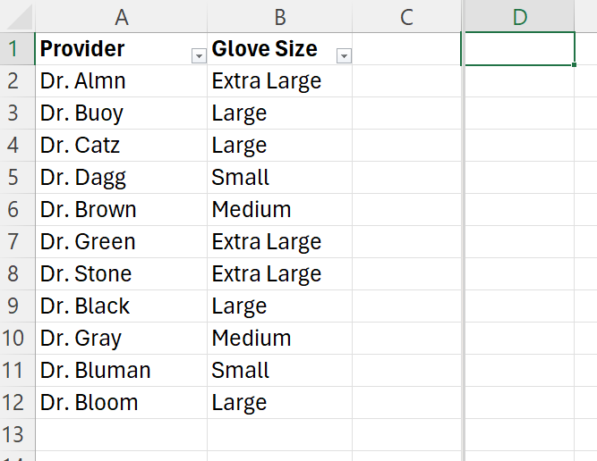
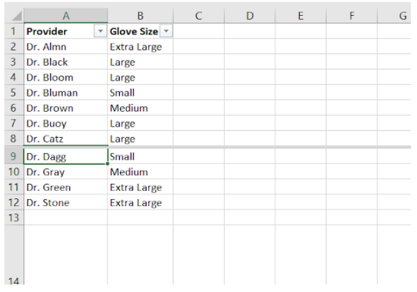
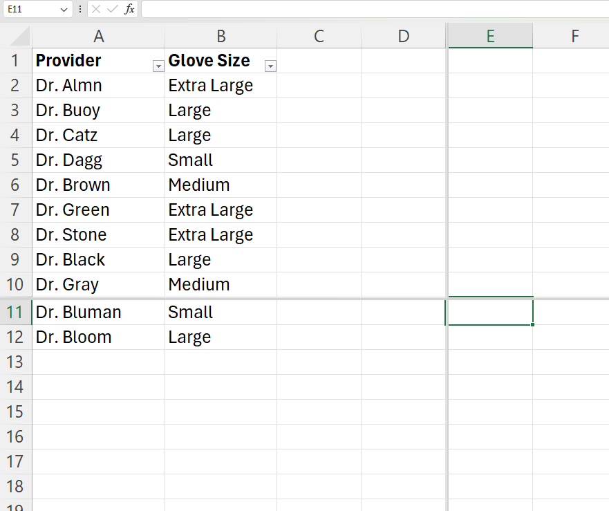
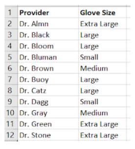
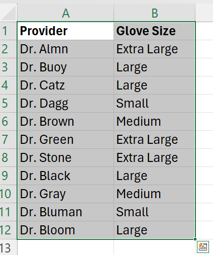
To sort a worksheet: Select a cell in the column to be sorted. Using the Data tab, select the desired command in the Sort & Filter group. The data will then be sorted based on the desired option. For instance, Figure 10C shows a list of providers and glove sizes. To alphabetize the providers, a cell is selected in Column A. The Sort A to Z command is selected in the Sort & Filter group on the Data tab. Figure 10D shows the completed sort. The information in each row remains together, but the location of the row may have moved higher or lower on the worksheet based on the sort.
Filtering Data
Filtering data helps the user find the desired data in the worksheet. To filter data in a worksheet, the columns must have headers.
To filter data in a worksheet: Select a cell in the header row. Using the Data tab, select the Filter command in the Sort & Filter group. Dropdown arrows will appear in each cell in the header row that has data. Select the header cell to be used for the filtering and click the down arrow. On the Filter menu, deselect (uncheck) Select All. Then, select the option(s) to filter by. Click OK. Only the rows containing the option(s) selected will show.
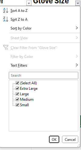
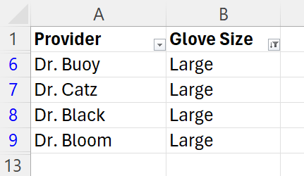
For example, in Figure 11A, the worksheet contains providers’ names and glove sizes. These titles appear in the header row (Row 1). Cell B1 was selected, and the Filter command was selected. The dropdown arrows appeared in each header row cell (Figure 11B). When the arrow is clicked, the Filter menu appears (Figure 11C). The lower portion of the menu contains the filtering options. Select All was deselected. (The box was clicked, and the checkmark disappeared.) Then, Large was selected and OK was clicked. Figure 11D shows the result of the filter.


To remove the filter or to see all of the data: Click the down arrow in the header row cell. Click the box next to Select All and the worksheet will show all of the data. Another option to clear the filter is to click on the Clear command in the Sort & Filter group on the Data tab (Figure 11E).
Create and Modify Tables
Excel contains tools to create professional looking tables. Predefined table styles are available to quickly create tables. Features can be added or removed from the table, quickly changing the appearance of the table.
Create Tables
Because a worksheet may contain data that will not be included in a table, the user must first select the cell range for the table.
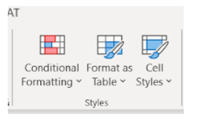
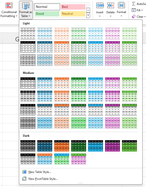
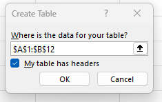
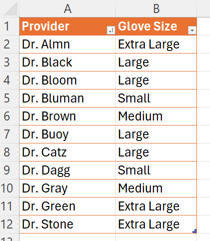
To create a table: Select the cells that will be part of the table. Using the Home tab, click the Format as Table command in the Styles group (Figure 12A). A dropdown menu appears. The names of the table styles appear when hovering over the style. Select the desired table style (Figure 12B). The Create Table dialog box appears (Figure 12C). Confirm the location of the data for the table and if the table has headers. Click OK. The table style is applied to the selected cells (Figure 12D).
Modify Tables
Once a cell range is formatted as a table, the user can modify the appearance of the table by using tools and commands on the Table Design contextual tab. When a cell in the table is selected, the Table Design contextual tab appears on the ribbon.
The Table Styles Options group on the Table Design contextual tab provides additional options to modify the table appearance (Figure 13A). These options include header row, total row, banded row, first column, last column, banded columns, and filter button (in the header row).
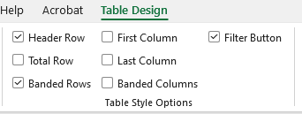
To change the appearance of the table: Select any cell in the table. Click on the Table Design contextual tab. Remove or add checkmarks as desired in the Table Style Options group. As the checkmarks are added or removed, the table is immediately changed.
To change the table style: Select any cell in the table. Using the Table Design contextual tab, select the More button in the Table Styles group (Figure 13B). Hover over the style to see it temporarily applied to the table. Click the desired style and it is applied to the table.

Remove a Table
A table can be removed without impacting the data in the cell range. The formatting of the table may or may not change, depending on the style applied.
To remove a table: Select any cell in the table. Using the Table Design tab, select the Convert to Range command in the Tools group. When the dialog box appears, click Yes to convert the table to a normal range.
Create and Modify Charts
Charts are used to present the data to the audience in an easy to visualize way. Excel contains tools to create a variety of charts. Each type of chart has variations, including 2D and 3D images. Table 5 shows a couple of the more commonly used Excel charts.
| Type | Description | Variations |
|---|---|---|
| Column charts | The data is represented in a vertical bar. Provides a comparison of the values for a few categories. |  |
| Bar chart | The data is represented in a horizontal bar. Provides a comparison of the values for a few categories. |  |
| Line chart | Used to show trends over time or categories. The data points form a line, which helps the audience view the trends. |  |
| Pie chart | Used to show the proportional comparison of the data. All the numbers add up to 100%. |  |
Chart Elements
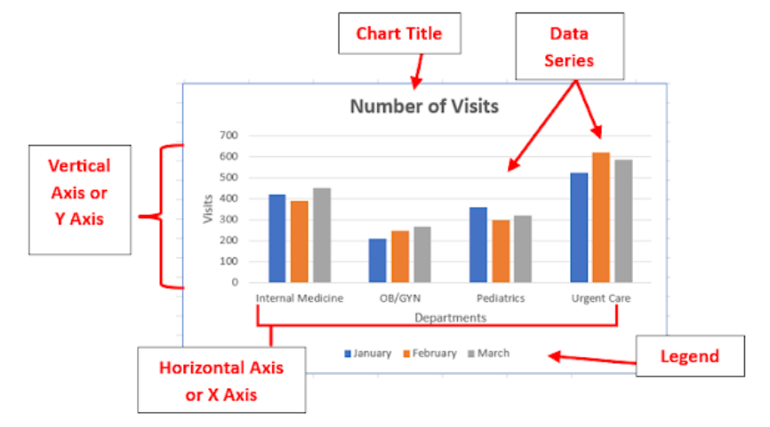
Charts contain these different elements (Figure 14):
- Vertical or Y axis: Measures the values of the columns. A vertical axis title may be present to the left of the values. (For example, in Figure 14A “Visits” is the vertical axis title.)
- Chart title: Provides information on what the chart is about.
- Data series: Shows the data points for each area.
- Legend: Provides a guide for each data series color on the chart.
- Horizontal or X axis: Provides information on the categories of the chart. A horizontal axis title may be below the category labels. (For example, in Figure 14A “Departments” is the horizontal axis title.)
Inserting and Modifying Charts
When a chart is inserted into a worksheet, the format can be modified.
To insert a chart: Select the cell range (including titles and row labels) to be inserted into the chart. Using the Insert tab, click a desired chart in the Chart group. When a menu displays, select the desired chart type.
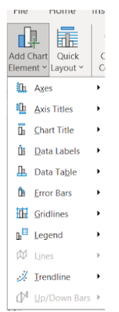
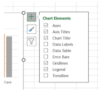
To add chart elements: A chart title, legend, and labels can be added to the chart. Click anywhere in the chart. Using the Chart Design tab (Figure 15A), click the Add Chart Element command in the Chart Layouts group. A dropdown menu will open (Figure 15B). Select the element and the desired option. Chart elements can be added or removed from the chart by clicking the plus sign (+) button at the side of the chart (Figure 15C). Some elements will add text box placeholders to the chart. Double-click the text box placeholder to add the information. Click outside the chart to close the text box.
To change the layout: Click anywhere in the chart. Using the Chart Design tab, click the Quick Layout command in the Chart Layouts group. A dropdown menu will open. Select the desired layout.
To change the color: Click anywhere in the chart. Using the Chart Design tab, click the Change Styles command in the Chart Styles group. A dropdown menu will open. Select the desired color.
To change the chart style: Click anywhere in the chart. Using the Chart Design tab, click the More button on the Chart Styles group. A dropdown menu will open. Select the desired style.
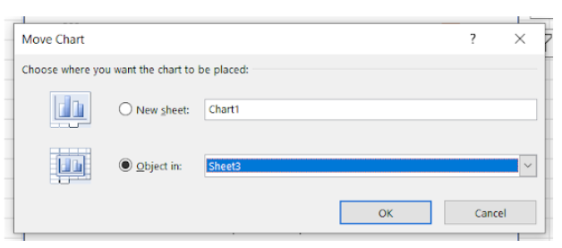
To move the chart on the worksheet: The chart will move like an object on the worksheet. Click and drag the chart to the desired location. To move the chart to another worksheet, select the chart. Using the Chart Design tab, select the Move Chart command in the Location group. The Move Chart dialog box will appear (see Figure 15D). Select the desired location for the chart and click OK.

Learning Activities
Excel Formulas, Functions, and Tables – Flash Cards
Application Exercise 1
Directions: Create a worksheet. Practice using formulas, functions, absolute reference, and relative reference. Create a table and apply a table style.
- Open a new Excel workbook and save as: Exercise 14 1
- Create the worksheet shown in Figure 15A.
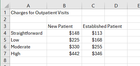
Figure 15A. Practice worksheet. - Apply the Accounting format to the cell range B4:C7. Use two places after the decimal and use the dollar sign ($).
- Using the cell range A1:C1, Center and Merge the title.
- Format the font in Row 1 by using Arial 14 pt bold font in an orange shade of your choice.
- In A3, type: Visit Type
- In E1, type: Increase:
- The charges will increase by 15%. In F1, type: 1.15
- Copy cell range B3:C3 and paste in E3. (Establish Patients should be in F3.)
- Create a formula in E4 that would multiple B4 and F1. Use B4 in the formula. Create an absolute reference for F1.
- Copy the formula in E4 and paste to cell range E5:E7.
- Copy the formula in cell range E4:E7 and paste to cell range F4:F7.
- Apply the Accounting format (with two digits after the decimal), if cell range E4:F7 is not formatted.
- In cell A9, type: Average Cost
- In cell A10, type: Minimum Cost
- In cell A11, type: Maximum Cost
- In cell A13, type: Number of Visit Types
- In cell B9, use the Average function to find the average cost of the new patient visits from cell range B4:B7.
- In cell B10, use the Min function to find the lowest cost of the new patient visits from cell range B4:B7.
- In cell B11, use the Max function to find the highest cost of the new patient visits from cell range B4:B7.
- In cell B13, use the Count Numbers function to find the total number of visit types for cell range B4:B7.
- Copy cell range B9:B11 and paste in C9:C11.
- Copy cell range B9:C11 and paste in E9:F11.
- Format the text in the cell range A4:A13 by using Arial 11 pt italic font.
- Format the font in Row 3 by using Arial 12 pt bold font and center font. Wrap text in cell range B3:F3.
- Format the font in the cell range B4:F13 by using Arial 11 pt.
- For E1, apply Align Right alignment to the cell.
- Select cell range A3:C7 and format as a table. Select a style of your choice. Remember your table has headers.
- Adjust column widths as needed to see the text.
- Save the workbook. Your worksheet should look like Figure 15B.
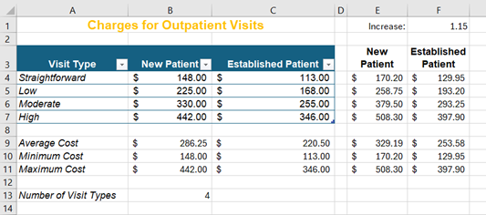
Figure 15B. Completed practice worksheet. - To check the formulas and functions used, click on the Formulas tab and select the Show Formula command in the Formula Auditing group. Your worksheet should look like Figure 15C.

Figure 15C. Completed practice worksheet showing the formulas and functions used.
A mathematical equation in a spreadsheet that performs a calculation and shows the result in a cell.
A single box on a table or spreadsheet that can contain text or numbers.
The independent variable of a function.
The horizontal series of cells separated by lines or space form other horizontal series of cells and found in a table or spreadsheet.
Any of two or more vertical sections of type on a document.
The cell reference changes when the formula is copied to another cell. Is also called relative cell reference.
The cell reference in the formula is constant (always use the same cell) even when it is copied to other cells. Is also called absolute cell reference.
A predefined formula in a spreadsheet that performs a calculation with specific values.
The top row of a table that contains the titles for the columns.
A rectangular grid consisting of columns and rows. Allows for an orderly arrangement of data.
Having strips or bands of contrasting colors.
Moving the mouse pointer over an option without selecting it.

